

What Calibration Coefficients Do
ASTM E74, ISO 376, and other standards may use calibration coefficients to characterize the performance characteristics of continuous reading force-measuring equipment better. These standards may use higher-order fits such as a second or third-order fit (ISO 376) or ASTM E74 allows higher-order fits up to as high as a 5th-order.
Both Standards use observed data, and they both fit the data to a curve. In simple terms, these higher-order fits give instructions on how best to predict an output given a measured input. This assumes multiple measured values of the force-measuring device are grouped closely together. When calibrating to a standard such as ASTM E74, or ISO 376, we often refer to this grouping as between run variance.
The higher the variance, the larger the reproducibility error in the standard uncertainty becomes, which raises the Lower Limit Factor (ASTM E74) or Reproducibility b (ISO 376). That output can either be the Force at a specific response or the Response when the Force is known.
We can use these equations to predict the appropriate coordinate more accurately for any point in the measurement range, typically above the first non-zero point on the curve. The ASTM E74 standard has additional requirements for higher-order fits.
To use a fit above the 2nd-degree (or quadratic) requires the force-measuring device to have a resolution that exceeds 50,000 counts. Almost any force-measuring device can be characterized using standard equations; many will remember from algebra classes they may have had in high school.
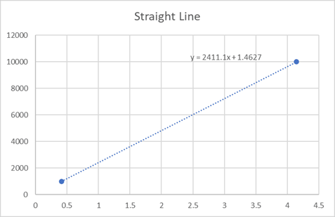
Figure 1 Load Cell Curve Using the Equation for a Straight Line Where Y - Values are Force and X -Values are Response (What the Instrument Reads).
Calibration Coefficients Straight Line Fits
Straight-line equations such as y = mx + b is common for force-measuring devices shown in Figure 1. One would typically find the slope of the line, which could predict other points along the line. The standard formula of y = mx + b, where m designates the slope of the line, and where b is the y-intercept that is b is the second coordinate of a point where the line crosses the y-axis.
We can modify this formula to use coefficients, and it would become Force = B1 * (Response) + B0. If we switched the x and y-axis, we would develop a formula for solving for Response = A1 * (Force) + A0 Figure 1 shows us a force-measuring device with consistent linear behavior.
Some devices may deviate from the line that we cannot precisely, or maybe we cannot predict precisely enough for the measurements we need to make. Thus, a straight line may introduce additional errors. It is often dependent on how linear the force-measuring device is to determine if a straight line gives us enough precision. Typically, this is characterized as nonlinearity; the error on most good force-measuring equipment is often less than 0.05 %.
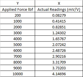
Figure 2 Data To Plot the Line in Figure 1 Which Would Produce B0 and B1 Coefficients
When we use this equation, y is the Force applied, and x is the output of the force-measuring device. If one wanted to solve for the output of the readings when they know the Force applied, they could decide to plot the actual readings against the Force applied, which is just changing what x is and what is y, or they can use the same formula and solve for x. To do this, we take the formula y = Mx + B and solve for x. The formula then becomes Mx = (y-B), which we then divide (y-B) by m. Thus, x = (y-B)/M.
Pretty simple, right? When we get to higher-order equations, the formulas get more complicated.
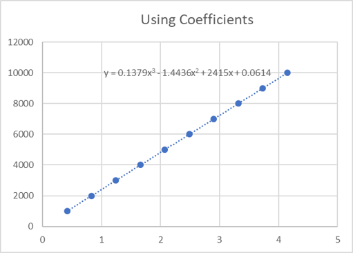
Figure 3 Using Least Squares Method or Higher-Order Equations
Calibration Coefficients Using Least Squares and Higher-Order Equations
Like a simple straight line, this regression analysis method begins with a set of data points that are plotted on an x- and y-axis graph. ASTM E74, ISO 376, and other standards use the method of least squares because it is the smallest sum of squares of errors.
It is the best approximate solution to an inconsistent matrix, often involving multiple x- values. The method used in ASTM E74 will contain a formula that is a bit more complex than a straight line. Section 7.1.2 of the ASTM E74 standard states, "A polynomial equation is fitted to the calibration data by the least-squares method to predict deflection values throughout the verified range of Force.
Such an equation compensates effectively for the nonlinearity of the calibration curve. The standard deviation determined from the difference of each measured deflection value from the value derived from the polynomial curve at that Force provides a measure of the error of the data to the curve fit equation.
A statistical estimate, called the lower limit factor, LLF, is derived from the calculated standard deviation and represents the width of the band of these deviations about the basic curve with a probability of approximately 99 %."[1] The polynomial equation often uses higher-order equations to minimize the error and best replicate the line.
Figure 3 above shows a plot from the actual readings in mV/V and fit to a 3rd-order equation. Instead of using the equation for a straight line (y=mx+b), we have a formula that uses x values that are raised to higher powers, such as Response(mV/V) = A0 +A1 * F + A2 * F2 where: A0 = 0.0614, A1 = 2415, A2 = -1.4436, and A3 = 0.17379. These are often called coefficients. On a calibration report, they are often referred to as A0, A1, A2, A3. Let us look at these numbers and dissect them from a calibration report.
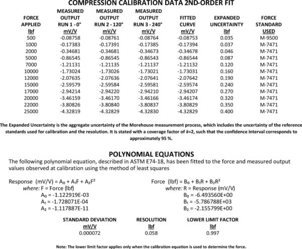
Figure 4 Calibration Report from Morehouse Showing a 2nd-degree Equation
The calibration coefficients shown in the report in Figure 4 show the formulas to solve for Response and an additional formula to solve for the Force. The formula for Force is found by switching the x- and y-axis, as discussed in the previous section. If you wanted to generate coefficients to solve for Force or find the B coefficients, you would use the Predicted Response for the x- values and Force for the y- values.
Morehouse has a spreadsheet available for download that will use these formulas to help interpolate values that are not on the certificate of calibration.
Note: Additional information on how to calculate the calibration equation is found in Section 8 of the ASTM E74 Standard titled Calculation and Analysis of Data. If using Microsoft Excel functions such as INDEX and LINEST are very useful tools for using the method of least squares.
One would first take the average of the three runs and then could use a formula @INDEX(LINEST(AVERAGE OF RUNS:OFFSET(AVERAGE OF RUNS,COUNT(FORCE APPLIED VALUES)-1,0),ZERO:OFFSET(ZERO,COUNT(FORCE APPLIED VALUES)-1,0)^{1,2,3,4,5}),6)
This example is for the 5th order polynomial, 4th Order would use the same formula ^{1,2,3,4}),5), 3rd order ^{1,2,3}),4), 2nd order ^{1,2}),3), ^{1}),2).
ASTM gives further guidance in Annex A1 on determining the degree of the best-fitting polynomial for high-resolution force-measuring instruments.
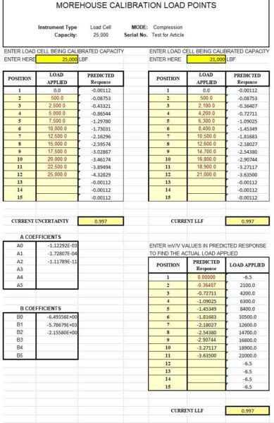
Figure 5 Morehouse Spreadsheet
The formula for Response is used when one knows the target force they wish to achieve and needs to know what the device will need to read at that point. For example, in reading the calibration certificate in Figure 4, if one wanted to apply 20,000 lbf of Force, one would load the force-measuring device until it would read -3.46174 mV/V.
However, if they would want to apply 21,000 lbf of Force, they would need to use the equation to solve for Force found above. This equation is Response = -1.122919E-03 + -1.728071E-11 * (21,000) + -1.117887E-11 * (21,000^2).
Thus, to generate 21,000 lbf, the device should read -3.63500 mV/V. Morehouse has developed a simple spreadsheet where anyone can generate load tables and plug these equations in to solve for either Force or Response.
Examining What the Calibration Coefficients Mean
A0 and B0 would be the constant at which the equation crosses the y-intercept.
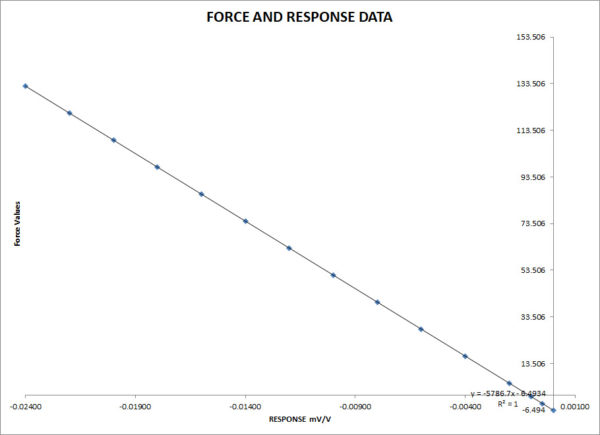
Figure 6 Shows the Relationship of Force versus Response at Very Low Responses
Many customers do not like this as many want to see 0 displayed on a device when they 0 the instrument. That is not how math works. In this example, when the meter reads zero, the force value will be -6.49365 lbf or sometimes a rounded number, which would be -6.5 lbf as B0 = -6.49356.
The reason for this is the equation is Force (lbf) is equal to B0 + B1 * (Response)+B2 * (Response^2). Simply put, B1, B2, and higher are multiplied by the 0 on the meter except for the first one. The meter will read 0.0 when the Response is equal to A0 or -0.00112 mV/V.
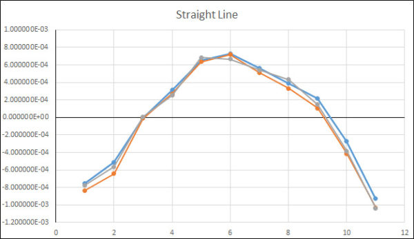
Figure 7 Deviation (Residuals) Between Actual Reading and Fitted Curve Using a Straight Line Fit
A1 * F and B1 * R is the linear term; in Figure 7 above, we are showing the deviations from the fitted curve, meaning we draw a straight line through all of the points and then subtract the predicted Response from the actual force-measuring device reading. We are using this method because if we showed three runs of data with very small changes, the lines would all blend, as shown in Figure 12.
When using a straight line, the deviations are much larger, and the overall reproducibility is less. The ASTM llf, which represents a large portion of the reproducibility error, jumps from 0.997 lbf, as shown in Figure 4, to 8.14 lbf, or about eight times worse.
Note: It is important to note that we are using one example for these graphs. The residual plots may vary depending on the exact measurements. So, when we say this plot is better than another, it is specific to this force-measuring device. Generally,higher-order equations will better replicate how the device performs when compared to a first-order equation.
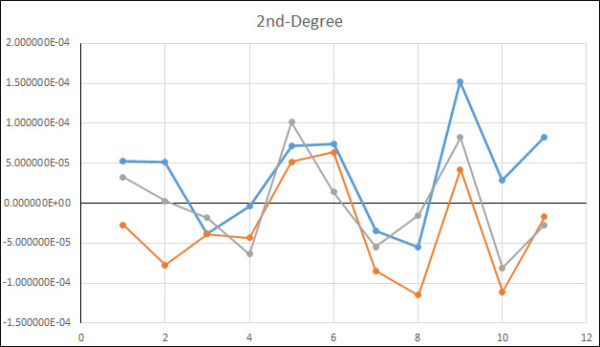
Figure 8 Deviation Between Actual Reading and Fitted Curve Using a Quadratic (2nd-Degree) Fit
A2 * F2 and B2 * R2 is the quadratic term
A positive quadratic coefficient causes the parabola's ends to point upward, while a negative cause quadratic coefficient causes the parabola to point downward. When we characterize the force-measuring device using a quadratic term, we have an ASMT llf of 0.997 lbf; this will be the 2nd best fit as only the Quintic will be a little better.
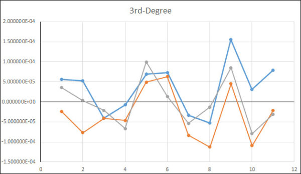
Figure 9 Deviation Between Actual Reading and Fitted Curve Using a Cubic (3rd-Degree) Fit
A3 * F3 and B3 * R3 is the cubic term. This coefficient functions to make the graph "wider" or "skinnier" or reflect it, if negative—the greater the calibration coefficient, the skinnier the graph. The cubic fit is a little worse than the quadratic by about 0.15 lbf.
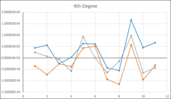
Figure 10 Deviation Between Actual Reading and Fitted Curve Using a Quartic (4th-Degree) Fit
A4 * F4 and B4 * R4 is the quartic term. These have zero to four roots, one, two, or three extrema, and zero, one, or two inflection points. There is often no general symmetry, and much more complicated to solve. There can be different inflection points, and they can have various roots. The Quartic fit is a little worse than the quadratic by about 0.17 lbf.
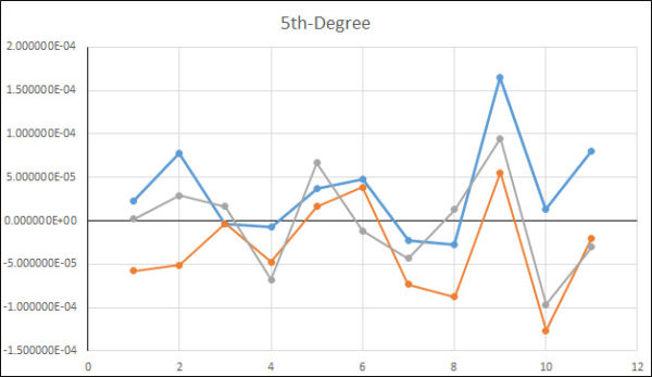
Figure 11 Deviation Between Actual Reading and Fitted Curve Using a Quintic (5th-degree) Fit
A5 * F5 and B5 * R5 is the quintic term. These have one to five roots, zero to four extrema, one to three inflection points, and no general symmetry. The Quintic fit is better than the quadratic by about 0.17 lbf.
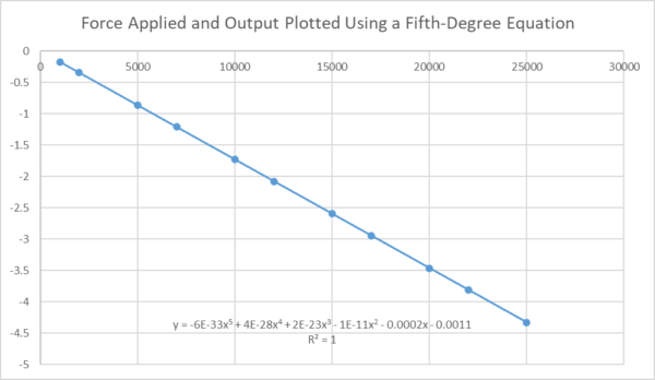
Figure 12 Shows the Plotted Values Versus the Force Applied.
Calibration Coefficients Conclusion
Higher-order equations allow the line to take on different forms to characterize the force-measuring device best. The equations are similar to instructions telling the line to turn up, down, have a parabola, be narrow or wide, and in which directions; since we are dealing with such small deviations, it is tough to see any of these behaviors on a graph as shown in Figure 12.
Suppose the force-measuring device is very repeatable but may not be as linear. In that case, the quartic or quintic function may best characterize the device producing a curve that may deviate at several points from linear behavior.
We see in Figure 12 the R-squared value is 1, meaning the curve coefficients best represent the line as R-squared is a statistical measure representing the proportion of the variance for a dependent variable that is explained by an independent variable or variables in a regression model.
The further R-squared is from 1, the larger the between-run variance becomes, increasing the overall uncertainty. Different standards have requirements that need to be met for higher-order equations.
Implementing good measurement practices, having deadweight machines with very low uncertainties, and following published standards allow Morehouse to produce data with repeatable results. We need to graph those deviations to show the actual behavior of the force-measuring device.
The coefficients may best characterize the force-measuring device's performance and allow the end user to predict what the device should read at specific force points along with the calibrated range.
The A0 and B0 calibration coefficients will never be zero unless we force them to be, which is not the intent of the standards, thus when the indicator displays 0, and one uses the equation, the value at 0 will be the B0 calibration coefficient.
I take great pride in our knowledgeable team at Morehouse, who will work with you to find the right solution. We have been in business for over a century and have a focus on being the most recognized name in the force business.
That vision comes from educating our customers on what matters most and having the right discussions, including helping them understand calibration coefficients.
If you enjoyed this article, check out our LinkedIn and YouTube channel for more helpful posts and videos.
Everything we do, we believe in changing how people think about Force and Torque calibration. We challenge the "just calibrate it" mentality by educating our customers on what matters and what causes significant errors, and focus on reducing them. Morehouse makes simple-to-use calibration products.
We build fantastic force equipment that is plumb, level, square, rigid, and provide unparalleled calibration service with less than two-week lead times.
Contact us at 717-843-0081 to speak to a live person or email info@mhforce.com for more information.
[1] ASTM E74-18
#Calibration Coefficients
About Morehouse Instrument Company Companies worldwide rely on Morehouse for accuracy and speed. The company turns around equipment in 7-10 business days so customers can return to work quickly and save money.
The York, PA-based company provides force and torque measurement products and services worldwide.
Morehouse Instrument Company, a trusted and accredited provider of force and torque measurement services for over 100 years, offers measurement uncertainties 10-50 times lower than the competition.
Morehouse helps commercial labs, government labs, and other organizations lower their measurement risk by lowering equipment uncertainties for torque and force measurement. Contact Morehouse at info@mhforce.com or www.mhforce.com
More Information about Morehouse
We believe in changing how people think about force and torque calibration in everything we do.
This includes setting expectations on load cell reliability and challenging the "just calibrate it" mentality by educating our customers on what matters and what causes significant errors.
We focus on reducing these errors and making our products simple and user-friendly.
This means your instruments will pass calibration more often and produce more precise measurements, giving you the confidence to focus on your business.
Companies around the globe rely on Morehouse for accuracy and speed.
Our measurement uncertainties are 10-50 times lower than the competition.
We turn around your equipment in 7-10 business days so you can return to work quickly, saving you money.
When you choose Morehouse, you're not just paying for a calibration service or a load cell.
You're investing in peace of mind, knowing your equipment is calibrated accurately and on time.
Contact Morehouse at info@mhforce.com to learn more about our calibration services and load cell products.
Email us if you ever want to chat or have questions about a blog.
We love talking about this stuff.
Our YouTube channel has videos on various force and torque calibration topics here.

