The GUM in Plain English, Part 4 of 7: Type B Uncertainty: The Doubt You Already Know

Part 3 earned four numbers by repeating measurements: our Type A pieces, led by a 0.58 lbf single-reading repeatability at 3 degrees of freedom. But not all doubt comes from repeating a measurement. Most of it, in a good lab, comes from things you already know and never re-measure.

You did not determine your reference standard’s uncertainty by running it four times this morning. You read it off the calibration certificate. You did not characterize your indicator’s resolution statistically. You read it off the front panel. That kind of evaluation, built from existing information rather than fresh repetition, is a Type B evaluation (GUM 4.3). It is not second-class. In this budget, the Type B pieces include the second-largest contributor of all.

The trick with Type B is turning what you know into a standard uncertainty, a one-sigma number you can combine with the rest. There are only a few moves, and they cover almost everything you will meet.

Divide a stated uncertainty by its coverage factor. When the information already comes as an uncertainty with a coverage factor, divide it back down. Our reference was calibrated by deadweight primary standards with a calibration and measurement capability (CMC) of 0.002 % of applied force, reported at k = 2. The CMC is the lab’s best case under ideal conditions; the uncertainty you report on a customer’s instrument is normally larger, because it also carries that instrument’s own doubt. At 5000 lbf, that is a 0.1 lbf expanded value. Divide by 2, and the standard uncertainty of the reference is 0.05 lbf. Done.

Turn a bound into a shape. When all you have is a bound, an “it cannot be off by more than this,” you have to assume a shape for the doubt inside the bound. If you have no reason to favor the middle over the edges, you assume every value is equally likely, a rectangular distribution, and divide the half-width by the square root of 3. Three of our inputs are sized this way. Reference standard stability: the reference shifted 0.01 % between its last two calibrations, which at 5000 lbf is a 0.5 lbf bound; rectangular, divided by √3, gives 0.29 lbf, the second-largest line in the whole budget, and it is pure Type B. Environmental factors: the cell’s temperature coefficient is about 0.0015 % per °C, and the lab holds the temperature to within 1 °C; that is 0.075 lbf at 5000 lbf; rectangular, divided by √3, gives 0.043 lbf. Other error sources: alignment is 1/16 in off the centerline, and the side-load sensitivity may be 0.05 % per inch, so the contribution is about 0.003 % of reading, or 0.15 lbf; rectangular, divided by √3, gives 0.087 lbf.

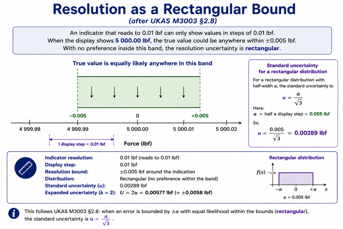
Figure 6. Resolution as a rectangular bound. An indicator reading to 0.01 lbf places the true value anywhere within one display step, so with no preference inside the band, the standard uncertainty is half a step divided by √3 (after UKAS M3003 §2.8).

Resolution is the same bound idea with a tighter step. The indicator resolves to 0.01 lbf at this point, the least increment of its display, so a reading can sit anywhere within that step. Divide by √12, which is just 2√3 for a half-step, and the resolution contribution is 0.0029 lbf. This is the oldest move in the Type B toolkit, and UKAS M3003 states it plainly: whenever a value is read off a finite display, there is always an uncertainty of plus or minus half the last increment (M3003, §2.8). A reading of 5000.00 lbf stands for any value from 4999.995 to 5000.005 lbf.

Why these particular divisors? They are just the standard deviations of those shapes, worked out once, so you do not have to. Here is the part the GUM points out and most people miss: the divisors land surprisingly close together, even though the shapes behind them demand wildly different amounts of knowledge to justify (GUM 4.3.9, note). The shape matters less than people fear. Picking a sensible bound matters far more.

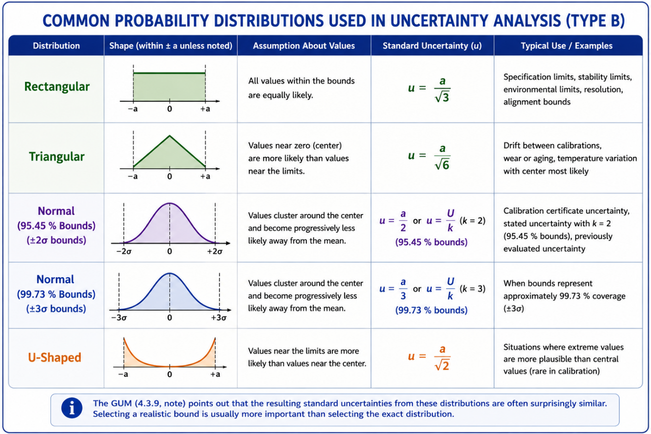
Figure 7. Common Type B probability distributions and their divisors: rectangular (÷√3), triangular (÷√6), normal at 95.45 % (÷2) and 99.73 % (÷3), and U-shaped (÷√2), with the assumption behind each.

Table 2. The Type B contributors for the 5000 lbf example, with the distribution assumed and the divisor that turns each bound into a standard uncertainty.

The GUM stopped using “random” and “systematic”

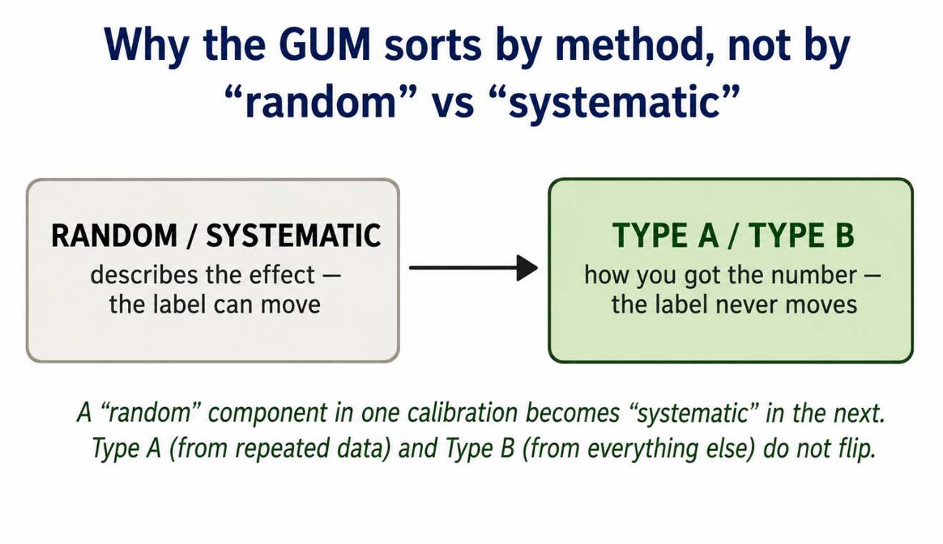
Figure 8. The GUM sorts by how you got the number, not by how the effect behaves. The label that flips is the one it dropped.

If you learned uncertainty before about 1993, you learned to sort errors into two bins: random and systematic. The GUM reserved those words for errors and removed them from uncertainty. People still trip on this, so here is what I’ve been told, as even though I remember Paul Harvey, I was in high school in 1993 and certainly not reading the GUM before 1999. And get this, I slept fine back then. Now I read the GUM and have issues staying asleep.

Random and systematic describe how an effect behaves. A random effect scatters your readings; average more, and it shrinks. A systematic effect pushes them all one way; averaging does nothing. Those are useful words for effects and for errors (GUM 3.2.2). They are bad words for uncertainty components, for one reason: the label moves. Calibrate a reference yesterday, and its scatter looked random. Use that reference today to calibrate a customer’s cell, and yesterday’s scatter is now a fixed offset baked into every reading, a systematic effect (GUM 3.3.3, note). Same number, different label, depending on how it is used. A classification that flips like that is no classification at all.

So the GUM sorts by a question that never flips: how did you get the number? If you got it from repeated data, it is Type A. If you got it from anything else, a certificate, a spec, a handbook, or judgment, it is Type B (GUM 3.3.3). That is the whole distinction.

Think of it as the artist formerly known as Prince. The music did not change when the name became a symbol nobody could pronounce. The catalog was the same; only the marquee changed, and people fumbled the new label for years. The GUM did the same thing to doubt. A reference-stability term off a certificate is the same number it always was. What changed is the question you ask to assign it.

This matters in practice for one reason above all. Both types are real uncertainty, both are standard deviations, and both go into the combination the same way (GUM 3.3.4). There is no penalty box for Type B and no gold star for Type A. The repeatability from four runs and the reference stability off a certificate sit side by side in the budget and add in exactly the same way. Which brings us to how they add.

Coming in Part 5: doubt does not add like money. It adds like the sides of a right triangle, and 3 plus 4 makes 5, not 7. We combine all nine inputs into one number, then meet the catch that most budgets quietly get wrong: correlation.

-Henry Zumbrun, Morehouse Instrument Company

Appendix: the formulas

Symbols are italic for quantities (U, k, u, s, n) and roman for units (N, kN, lbf). The combined standard uncertainty is u_c, and degrees of freedom is ν.

Standard uncertainty from repeated readings (Type A). For n repeated readings with experimental standard deviation s, the dispersion of a single reading is s itself; the standard uncertainty of their mean is u = s / √n. In force calibration, the repeatability carried is usually s, the doubt in a single determination, not s / √n.

Type B from a stated coverage factor. u = U / k.

Type B from a bound of half-width a. Rectangular: u = a / √3. Triangular: u = a / √6. Normal 99.73 % bound: u = a / 3. Normal 95.45 % bound: u = a / 2. U-shaped: u = a / √2.

Combined standard uncertainty. For independent inputs, root-sum-of-squares: u_c(y) = √[ Σ ( ci × u(xi) )² ]. With correlation, add a covariance term under the root; for perfectly correlated inputs the result reduces to a straight sum.

Expanded uncertainty. U = k × u_c(y).

Effective degrees of freedom (Welch-Satterthwaite). ν_eff = u_c(y)⁴ / Σ [ ui(y)⁴ / νi ]. Truncate to the next lower integer, then take k as the t value at your confidence level for that ν_eff.

Selected t values at 95 % confidence (NIST Technical Note 1297, Table B.1).

Worked combination for the running example. u_c = √(0.58² + 0.29² + 0.10² + 0.087² + 0.05² + 0.043² + 0.032² + 0.0029² + 0.006²) lbf = 0.666 lbf. The fourth-power sum is dominated by repeatability, 0.58⁴ / 3, so ν_eff ≈ 5.2, truncated to 5. U = 2.57 × 0.666 lbf = 1.71 lbf (0.0342 %).

References for the series: JCGM 100:2008 (the GUM) and Amendment 1:2026; JCGM 101:2008 (Monte Carlo); JCGM GUM-5:2026 (examples); JCGM 200:2012 (the VIM); NIST Technical Note 1297 (1994); ISO/IEC 17025:2017, Clauses 7.6 and 7.8.6; ASTM E74; UKAS M3003 Edition 6 (2024); NIST SP 811 (2008).

About Morehouse   

We believe in changing how people think about Force and Torque calibration in everything we do, including, "The GUM in Plain English, Part 4 of 7: Type B Uncertainty: The Doubt You Already Know"

This includes setting expectations and challenging the "just calibrate it" mentality by educating our customers on what matters and what may cause significant errors. 

We focus on reducing these errors and making our products simple and user-friendly. 

This means your instruments will pass calibration more often and produce more precise measurements, giving you the confidence to focus on your business. 

Companies around the globe rely on Morehouse for accuracy and speed. 

Our measurement uncertainties are 10-50 times lower than the competition, providing you with more accuracy and precision in force measurement. 

We turn around your equipment in 7-10 business days so you can return to work quickly and save money. 

When you choose Morehouse, you're not just paying for a calibration service or a load cell. 

You're investing in peace of mind, knowing your equipment is calibrated accurately and on time. 

Through Great People, Great Leaders, and Great Equipment, we empower organizations to make Better Measurements that enhance quality, reduce risk, and drive innovation. 

With over a century of experience, we're committed to raising industry standards, fostering collaboration, helping with understanding risk, and delivering exceptional calibration solutions that build a safer, more accurate future. 

Contact Morehouse at info@mhforce.com to learn more about our calibration services and load cell products. 

Email us if you ever want to chat or have questions about a blog. 

We love talking about this stuff. We have many more topics other than, "The GUM in Plain English, Part 4 of 7: Type B Uncertainty: The Doubt You Already Know"

Our YouTube channel has videos on various force and torque calibration topics here.