RSS vs. Welch–Satterthwaite: What Your Coverage Factor Is Really Promising

Ask ten calibration labs how they combine an uncertainty budget, and nine will say "RSS." Ask the same ten how they pick the coverage factor, and most will say "k = 2, for 95 %." The confidence in that nine out of ten is 90 %, give or take a lot: the exact 95 % interval runs from about 56 % to 99.7 %, because ten labs is a sample of ten. Acting sure on small samples is, conveniently, the subject of this article. Both answers are half right, and the missing half is where certificates quietly over-promise and under-deliver. This article lays out the two approaches the way the GUM frames them, works the arithmetic on textbook cases, and then runs five Morehouse CMC budgets, 57 force points in all, through both methods to show exactly when the difference is cosmetic and when it is not.

This article is the second, deeper half of a pair. The companion paper, The GUM in Plain English, explains measurement uncertainty in plain language and builds a real force-calibration budget one piece at a time; it is available as a free download at mhforce.com. Readers who want the gentler on-ramp should start there, then come back for this closer look at the coverage factor.

1. Two Steps, Not Two Methods

The phrase "RSS versus Welch–Satterthwaite" is common among calibration laboratories and slightly misleading, because the two are not rivals. They answer different questions, and the GUM asks both.

Step one is combination. Each input X_i carries a standard uncertainty u(x_i). For a linear model with independent inputs, the combined standard uncertainty is the root-sum-of-squares of the sensitivity-weighted contributions (GUM 5.1.2, Equation 10):

u_c²(y) = Σ c_i² u²(x_i)

That is RSS. Every method in this article uses it. Inside the GUM framework there is no alternative to it, short of the Monte Carlo method of JCGM 101:2008.

Step two is coverage. The combined standard uncertainty is a one-sigma figure, and a certificate reports an expanded uncertainty U = k × u_c(y) that is meant to bound the measurand with a stated coverage probability (GUM 6.2.1). The entire question is what k to use. The GUM is explicit that k depends on the probability distribution of the output quantity and on how well that distribution is known (GUM 6.3.1, 6.3.2). When the distribution is normal and u_c(y) itself is well determined, k = 2 gives about 95 % and k = 3 about 99 % (GUM 6.3.3). The phrase "well determined" is the hinge on which the whole door swings, and it is a smaller hinge than most people assume. A standard uncertainty computed from a handful of readings is not well determined, and the GUM's answer to that case is Annex G.

What calibration labs call "Welch–Satterthwaite" is the same RSS combination followed by the Annex G procedure: estimate the effective degrees of freedom ν_eff of u_c(y), look up the Student t factor for the chosen coverage probability at that ν_eff, and use it as k (GUM G.4.1, G.6.4). When ν_eff is large, t collapses to the normal factor and the two methods agree. When ν_eff is small, they do not.

That last sentence is the entire point of this article, and it deserves the volume. When ν_eff is small, k = 2 stops being a safe convention and becomes an overstatement: the certificate claims 95 % coverage that the data cannot support. Everything that follows, from the textbook cases to the 57 force points, measures how big that overstatement gets and shows how cheaply it is fixed.

The GUM's preferred method is the second one. G.6.4 states it directly: the coverage factor should be obtained from the t distribution at ν_eff, and the result reported with the coverage probability and ν_eff alongside it. The k = 2 convention is presented in G.6.6 as acceptable only when the conditions for the Central Limit Theorem hold and ν_eff is large enough that the difference is negligible. Annex G also notes that in practice k = 2 is commonly used and should be stated as such, so that the reader knows the coverage probability is approximate rather than computed.

A note on reading certificates. On a calibration certificate from Morehouse, NIST, or any accredited laboratory, the expanded uncertainty statement is required by ILAC-P14 (clause 5.2: the value, the coverage factor, and the coverage probability all go on the certificate), and the machinery behind it is the same RSS and coverage procedure described here. No sugar coating, though: that number is the expanded uncertainty at the time of calibration, under the laboratory's conditions. By design it covers the short-term contributions during calibration and the customer's device (clause 5.4), and it leaves out your operators, your environment, your machines, and the instrument's stability and drift in use. As anything more than a quick check, the certificate value is not your measurement uncertainty; it is one input to a budget you still have to build with many more inputs. Speaking of drift, I used to think I had the greatest joke about it, though it was so great that it changed very little over time. Ba dum tss.

One more point of GUM housekeeping. Both Type A and Type B components carry degrees of freedom. A Type A component from n independent readings carries n − 1 (GUM G.3.3). A Type B component carries whatever reliability you can defend for its bound; the GUM offers the relation ν_i ≈ ½ [Δu(x_i)/u(x_i)]⁻² (GUM G.4.2), so a bound you trust to 10 % carries about 50 degrees of freedom. The Morehouse workbooks assign 200 to Type B terms, which is large enough to be effectively infinite but still finite, so the fourth-power sum in Welch–Satterthwaite never divides by zero.

In plain words. Building an uncertainty has two steps. First you add up all the little doubts the right way, which is the square root of the sum of the squares, or RSS. Everybody does that. Second you multiply by a number k to stretch the answer so it covers about 95 % of the possibilities. Most people just use k = 2. The GUM says k = 2 is fine only if you had plenty of data. If you only measured something three or four times, you do not know your doubt very well, and k has to be bigger. Welch–Satterthwaite is the formula that tells you how much bigger. Also, the expanded uncertainty on your calibration certificate is only a starting point.

2. The Arithmetic

The Welch–Satterthwaite formula (GUM G.4.1, Equation G.2b) is

ν_eff = u_c⁴(y) / Σ [ u_i⁴(y) / ν_i ]

where u_i(y) = |c_i| u(x_i) is the contribution of input i in the units of the result, and ν_i is its degrees of freedom. Truncate ν_eff to the next lower integer, then take k = t_p(ν_eff) from the t table at the coverage probability p (GUM Table G.2). In short, ν_eff is how much data the whole budget effectively rests on: the formula reads the budget and reports a number of degrees of freedom, and the t table converts that number into the coverage factor k.

The formula looks dense, but three properties of it explain everything that follows.

The fourth power makes it a dominance test. A contribution that is 60 % of u_c contributes (0.6)⁴ ≈ 13 % of u_c⁴ to the numerator but, if it carries 3 degrees of freedom, dominates the denominator. A contribution at 20 % of u_c contributes (0.2)⁴ ≈ 0.2 %, and with 200 degrees of freedom it vanishes. Welch–Satterthwaite is a search for one thing: is there a large term that rests on little data? The fourth power filters the budget down to its biggest terms, and the division by ν_i asks how much data each of those terms carries. Small terms drop out of the question entirely, because their fourth power is negligible, and well-measured terms drop out too, because dividing by 200 leaves almost nothing. What survives is exactly the dangerous combination: big and thinly measured.

It is bounded below by the weakest term. Because Σ u_i⁴/ν_i ≤ (1/ν_min) Σ u_i⁴ ≤ u_c⁴/ν_min, the result satisfies ν_eff ≥ ν_min. The budget can never carry fewer degrees of freedom than its least-trusted component. It can carry far more, which is why the common shortcut of using the repeatability term's own n − 1 as the budget's degrees of freedom is wrong in both directions: it ignores the lift from the other terms and, when a well-known term dominates, it understates ν_eff badly. In plain terms, the budget can be no worse than its weakest line, and it is usually much better, because every additional line lifts it.

The penalty is steep near the origin and flat past 30. Table 1 gives the t factor at the two coverage probabilities calibration labs actually use. Note the convention: k = 2 corresponds to 95.45 % for a normal distribution, so that is the honest comparison. The GUM in Plain English used 95 % and k = 2.57 at 5 degrees of freedom; at 95.45 % the same budget gives 2.65. The shape of the table is the message. Below 10 degrees of freedom, every row changes k noticeably. Past 30, the rows barely move, and the two columns never differ by much. The row you are in matters far more than the column you read.

Table 1. Student t coverage factors against degrees of freedom.

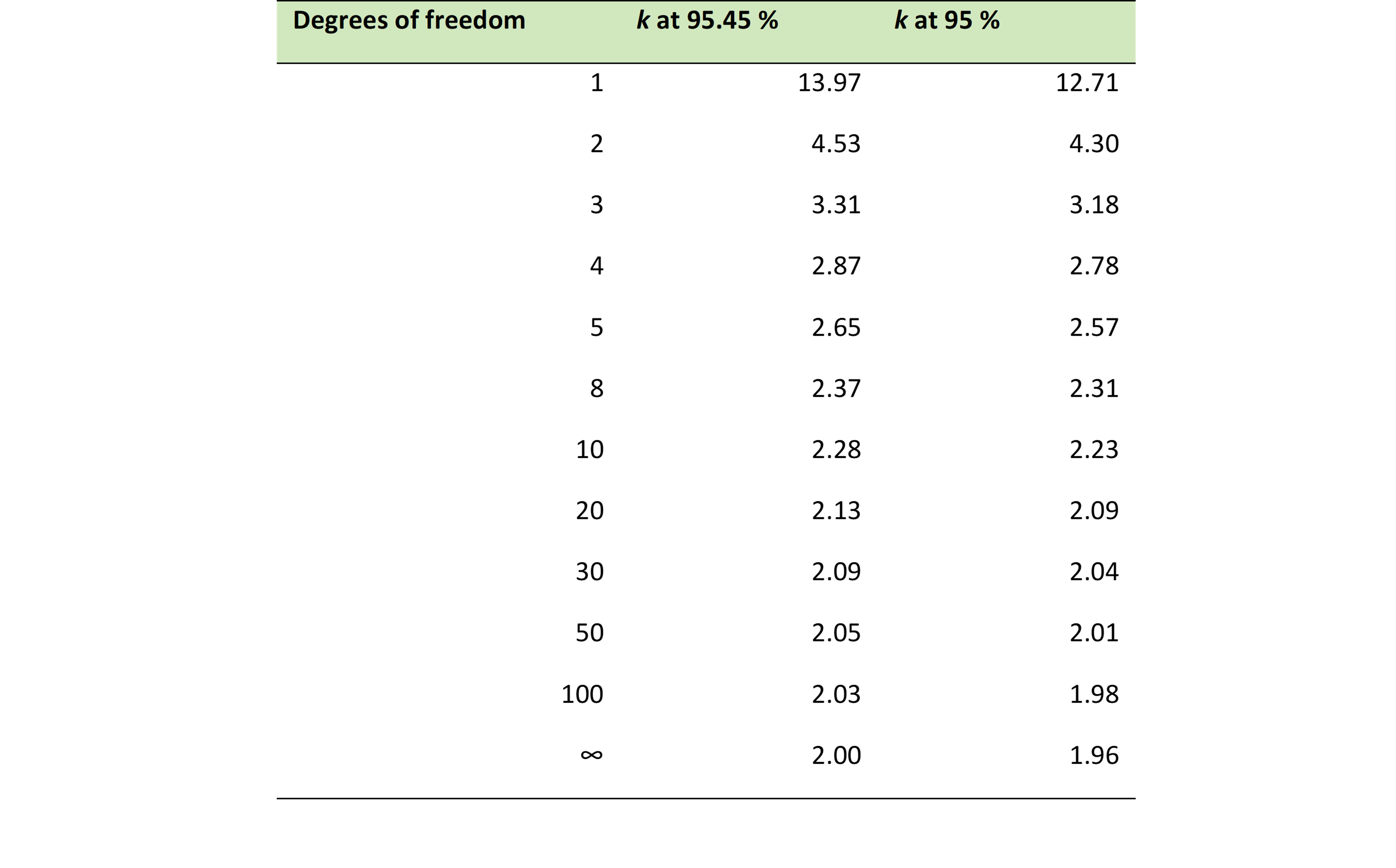
Figure 1. The coverage factor at 95.45 % against effective degrees of freedom. Above about 30 the curve sits within 4 % of k = 2. Below 10 it climbs fast, and at 2 or 3 degrees of freedom k = 2 is not a rounding error, it is a different claim.

In plain words. The formula raises each contributor to the fourth power, so the biggest contributor matters far more than everything else. The question it really asks is: did you measure your biggest contributor enough times? If you took 30 or more readings, k = 2 is close enough. ASTM E74 gets you there by design, since it requires multiple runs and at least 30 applied forces in a calibration. If you took three, the multiplier is 4.5, more than double. The chart shows the cliff.

3. Textbook Cases

Four small budgets, all in the same arbitrary unit, show the pattern before any force data enters. Each Type B term is treated as effectively infinite in degrees of freedom.

Table 2. Four textbook budgets at 95.45 % coverage. W–S: Welch–Satterthwaite.

Case 1 is the pure case. Three readings give two degrees of freedom, and the 95.45 % t factor at 2 degrees of freedom is 4.53. A lab that reports k = 2 on that budget has claimed a 95 % interval and delivered roughly an 82 % one. Nobody builds a one-line budget, but every budget with a dominant three-run repeatability term behaves like Case 1 to the degree that term dominates.

Case 2 adds a Type B term the same size. The combined uncertainty rises by √2, which is what RSS does, but the effective degrees of freedom rise from 2 to 8, which is what Welch–Satterthwaite does: the fourth-power ratio (1.414/1.0)⁴ = 4 multiplies the 2 degrees of freedom. The penalty falls from 126 % to 18 %. Adding a well-known term to a budget does not just enlarge it; it stabilizes it.

Case 3 shows the effect of more readings. Ten runs instead of three, with a Type B term half the size, lands at 14 effective degrees of freedom and a 10 % penalty. Still not negligible on a certificate, but survivable.

Case 4 is the reassuring one. When the thinly sampled term is small, Welch–Satterthwaite says so: a three-run term at 30 % of the Type B term gives 293 effective degrees of freedom, and k = 2 is correct to three figures. This is the case most labs assume they are in. The Morehouse data in the next section show how often they are not.

In plain words. When the biggest contributor rests on only three measurements, k = 2 can be off by more than double (Case 1). If you add other well-known contributors to the overall measurement uncertainty, the problem shrinks (Case 2). Measuring more times shrinks it too (Case 3). And if the three-measurement contributor is small compared with the others, there is no problem at all (Case 4). The formula sorts out which situation you are in. Guessing does not.

4. Five Morehouse CMC Budgets, 57 Force Points

The real test is a working budget. Morehouse builds a CMC budget at every calibration point of every reference standard it maintains, in a workbook (free for anyone to download from mhforce.com) that carries a degrees-of-freedom column on every line, computes ν_eff by Welch–Satterthwaite, and takes k from the t distribution at 95.45 %. That means every one of those budgets already contains both answers: U with k = 2 is simply 2u_c, and U as reported is t(ν_eff) u_c. The comparison below recomputes both from the component standard uncertainties and degrees of freedom in five of those workbooks, so that all five sit on the same 95.45 % convention.

Table 3. The five budgets.

Type B terms in every budget (reference standard stability, resolution of the unit under test, reference resolution, environmental conditions, miscellaneous error, and the reference laboratory's CMC) carry 200 degrees of freedom.

4.1 The Headline Result

Across all 57 points, if k = 2 were used instead of the calculated coverage factor, the expanded uncertainty would be under-reported by less than 2 % at 37 of them, by 2 % to 5 % at 4, by 5 % to 20 % at 10, and by more than 20 % at 6. The six large misses all have the same anatomy: single-point repeatability from three or four runs is the largest term in the budget, and it holds 50 % to 98 % of the variance. At those points the reported uncertainty would likely come down by taking more repeatability runs: each added run raises the degrees of freedom on the dominant term, which lowers k and, with it, the reported U. Figure 2 shows two of the five instruments point by point; Figure 4 shows all 57.

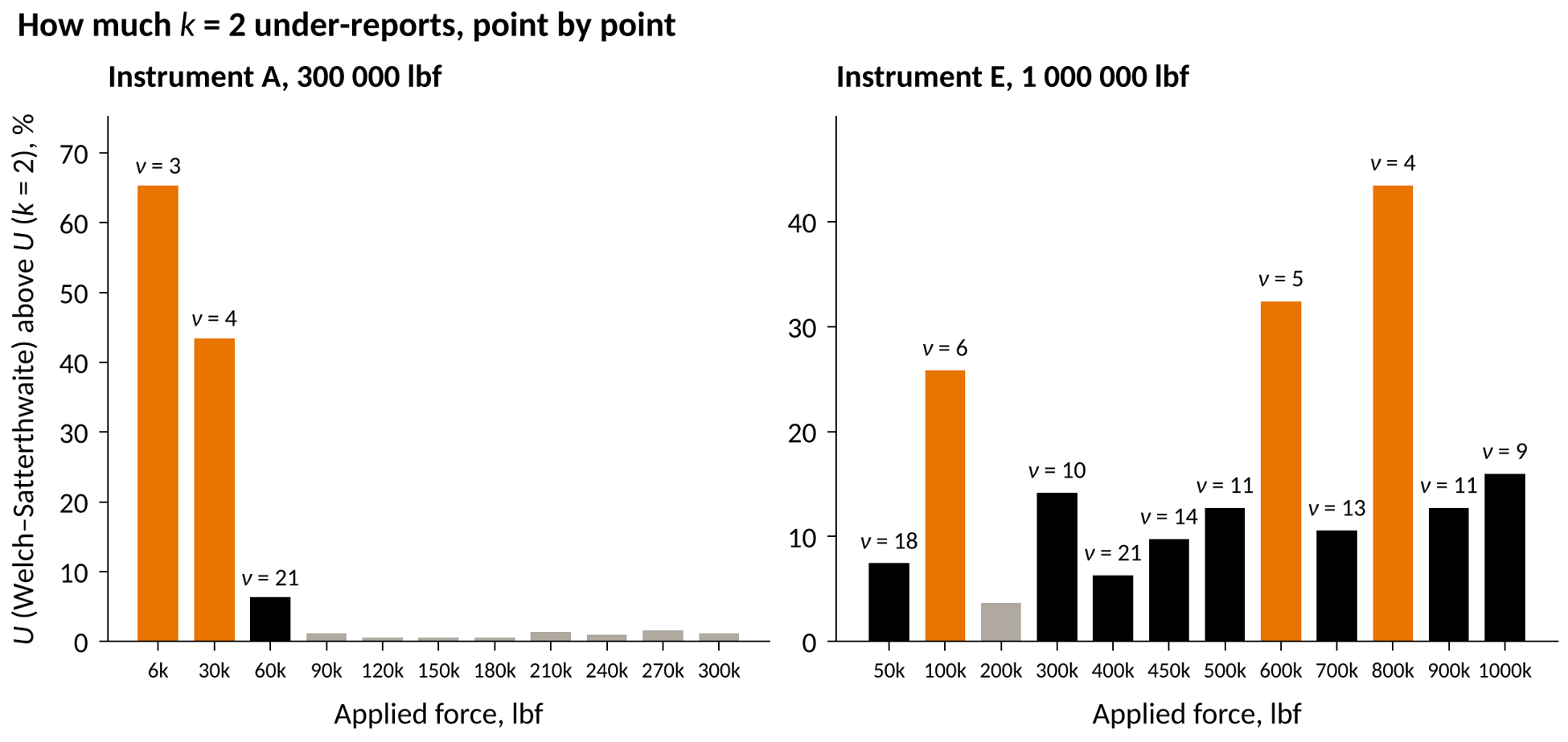
Figure 2. The percentage by which U from Welch–Satterthwaite exceeds U with k = 2, at every force point of Instruments A and E. Orange bars are 20 % or more, black bars 5 % to 20 %, grey bars under 5 %. The label on each bar is the truncated effective degrees of freedom.

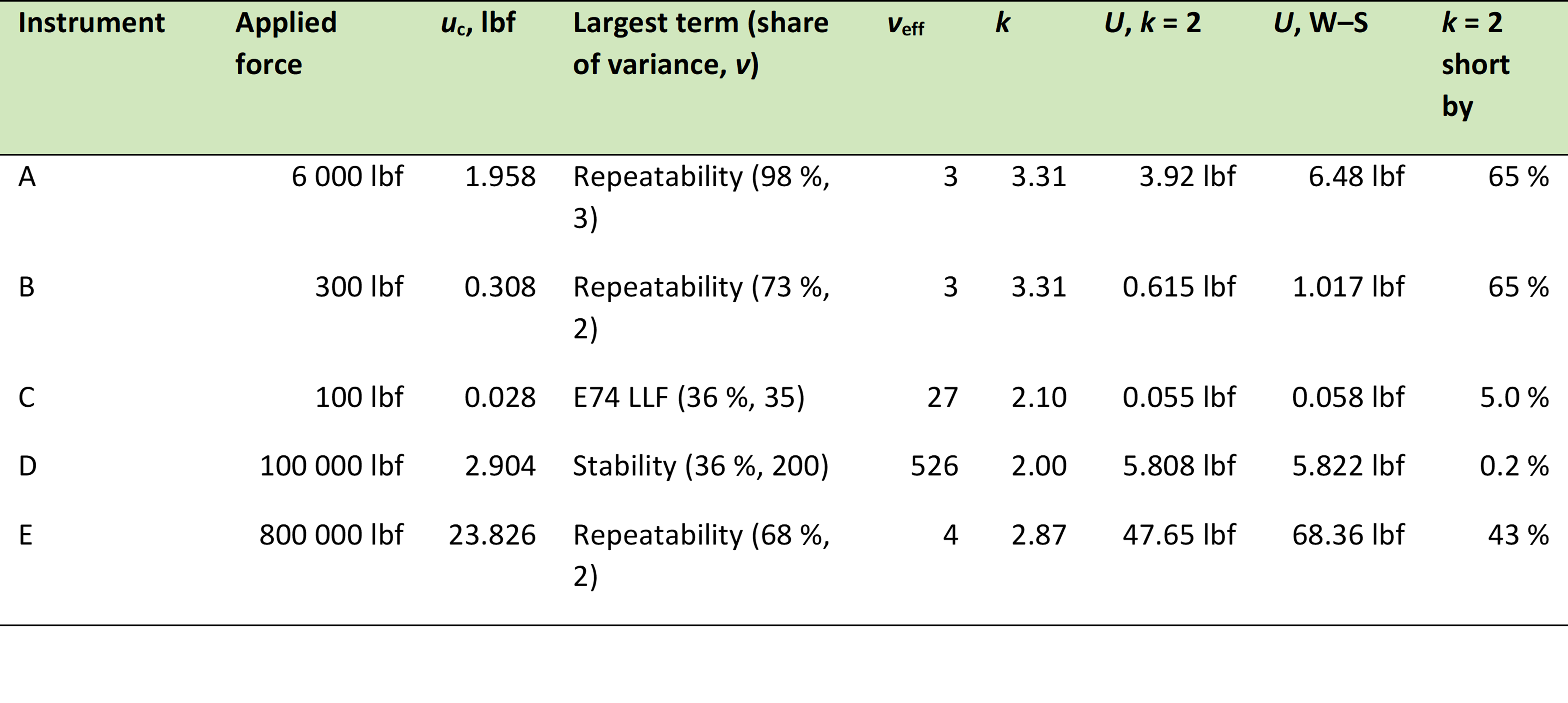
Table 4. One representative force point per instrument, both methods, 95.45 % coverage. W–S: Welch–Satterthwaite.

4.2 Where the Two Methods Agree

Instruments C and D never miss by more than 5 %, and their median miss is under 1 %. The reason is in Table 3. Both carry an ASTM E74 lower limit factor term with 32 or 35 degrees of freedom, and across most of the range the largest term is reference standard stability, a Type B term at 200. The three-run repeatability term is present at every point, but it is small compared with those two, so it falls into Case 4 of the textbook section. The repeatability term is still thin; it just does not matter.

Instrument B is the same story from the second point onward. At 500 lbf the LLF carries 75 % of the variance with 32 degrees of freedom, and ν_eff is 55. From 9 000 lbf up, the technician repeatability term at 18 degrees of freedom is the largest, and ν_eff sits above 90. Across those eleven points, k = 2 is never more than 2.3 % low.

Instrument A agrees from 90 000 lbf up, where stability dominates and ν_eff runs from 80 to 240. The miss is between 0.5 % and 1.6 %, which is below the rounding of a two-figure certificate value.

4.3 Where They Do Not

Instrument A at 6 000 lbf, its first point, is the clearest case in the set. Four runs gave a single-point repeatability of 1.936 lbf, which is 98 % of the variance; everything else in the budget totals 0.29 lbf. With ν = 3 on that term, ν_eff truncates to 3, k = 3.31, and the honest expanded uncertainty is 6.48 lbf rather than 3.92 lbf. That is a 65 % difference, and it is the difference between a certificate that means what it says and one that does not. At 30 000 lbf the same term holds 78 % of the variance and the miss is 43 %. By 60 000 lbf the stability term has grown with the applied force, repeatability has fallen to 37 % of the variance, and the miss drops to 6 %.

Instrument B at 300 lbf, its first point at 1 % of capacity, behaves the same way: three runs, 73 % of the variance, ν_eff = 3, 65 % miss. One point later, the LLF takes over and the problem is gone.

Instrument E is different and more instructive. It is a 1 000 000 lbf compression budget with three runs at every point and a fit standard deviation of 10.4 lbf at 32 degrees of freedom. At four of its twelve points the three-run repeatability is the largest term, and there the misses are 26 %, 32 %, 43 % and 16 %. But Instrument E never gets to the comfortable zone either. Even where the fit term dominates, repeatability is large enough that ν_eff stays between 10 and 35, and the miss stays between 4 % and 14 %. The median across all twelve points is 13 %. Figure 3 shows what the two methods look like on a certificate for Instrument A; the same plot for Instrument E would have the two curves separated along the entire range.

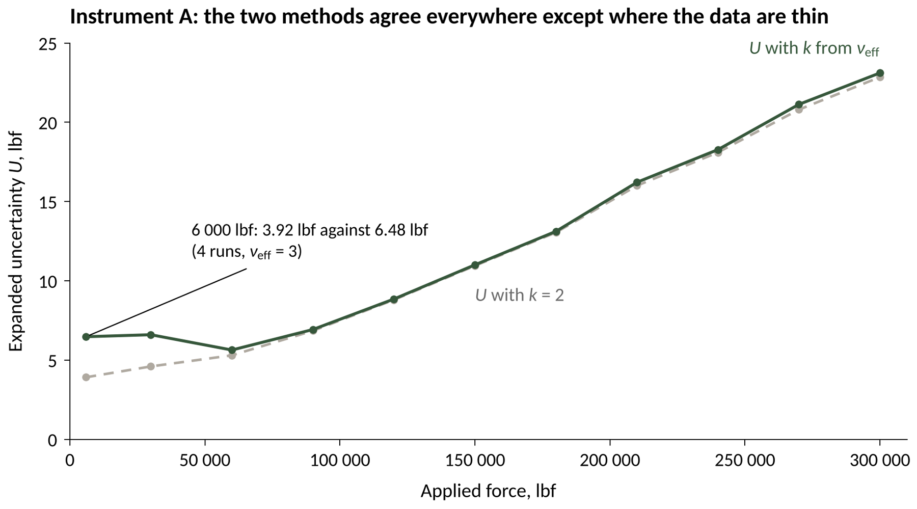
Figure 3. Instrument A, both methods. From 90 000 lbf upward the curves are indistinguishable at certificate resolution. At the first two points, the k = 2 line claims a 95 % interval the data cannot support.

Instrument A is a 300 000 lbf load cell calibrated by NIST with an ASTM E74 lower limit factor of 6 lbf. As reference standards go, it is beyond excellent, which is what makes its first two points such a clean illustration: nothing else in the budget is big enough to rescue a thin repeatability term.

Figure 4. All 57 force points. The miss is a function of ν_eff alone, and ν_eff is a function of how much of the variance rests on the three- or four-run repeatability term. The grey curve is t_95.45(ν_eff)/2 − 1. Past 30 effective degrees of freedom there is nothing to argue about.

4.4 What the Data Say About the Shortcut

Instrument A at 6 000 lbf also illustrates the shortcut mentioned in Section 2. Had the budget used the repeatability term's own ν = 3 directly, it would have reached the same k = 3.31, because that term holds 98 % of the variance and ν_eff truncates to 3 either way. At 30 000 lbf the shortcut would still say 3 while Welch–Satterthwaite says 4.9, truncated to 4: k = 2.87 rather than 3.31, a 15 % difference in the reported U. At 60 000 lbf the shortcut would say 3 and the formula says 21. The shortcut is only right when it does not matter which method you use.

In plain words. We checked 57 real force points. At 37 of them, using k = 2 would have been fine, off by less than 2 %. At 6 of them it would have been off by 20 % to 65 %. Every one of those six had the same cause: the biggest doubt came from measuring only three or four times. The lowest force point on an instrument is the usual place it happens, because the other doubts are tiny there and the repeatability stands alone. If you fix the low point by taking more readings, or if the other doubts are bigger, the problem goes away by itself.

5. What This Means on a Certificate

Report what the GUM asks for. A complete expanded uncertainty statement gives U, k, and the coverage probability (GUM 7.2.3), and when ν_eff is small enough to move k, gives ν_eff too (GUM 7.2.7, G.6.4). A certificate line that reads "U = 6.48 lbf, k = 3.31, 95.45 %, ν_eff = 3" tells a reader everything, including that the lab took four readings. The same line with k = 2 and U = 3.92 lbf tells them something that is not true.

NIST's own guidance lands in the same place. Technical Note 1297 carries the Welch–Satterthwaite formula and a Student t table in its Appendix B, and its successor, the Simple Guide of NIST Technical Note 1900 (2015), uses Student t coverage factors in its worked examples whenever the estimate rests on a few readings rather than defaulting to k = 2.

The direction of the error is always the same. Welch–Satterthwaite never returns k below the normal factor. Using k = 2 can only under-report. In conformity assessment, under-reported uncertainty means a test uncertainty ratio that looks better than it is and a guardband that is narrower than it should be. Instrument A at 6 000 lbf, reported with k = 2, would claim a TUR 65 % higher than the data support. A decision rule built on that number is built on sand, and those castles made of sand will wash away at high tide. I had to work in a Jimi Hendrix song title this time.

The fix is cheap, and it is not a bigger k. The point of carrying degrees of freedom is not to inflate U. It is to find the term that needs more data. On Instrument A, a fifth and sixth run at the first two points would move ν from 3 to 5, ν_eff from 3 to 5, and k from 3.31 to 2.65. Ten runs would bring k to about 2.3. Alternatively, sizing repeatability from the E74 fit across the range, as Instruments B through D do, brings 32 degrees of freedom to the term and solves the problem at every point. Either way, the choice is visible only because the budget carried the degrees of freedom in the first place. More labs should consider adopting ASTM E74 or E2428 for their force and torque standards. Those practices do a lot more than a commercial calibration on several fronts, degrees of freedom and expected performance among them, because they characterize the equipment under reproducibility conditions.

When ν_eff is large, say so and move on. Nothing in this article argues against k = 2. Forty-one of the 57 points are within 5 % of it, and the GUM itself says k = 2 is appropriate when the conditions hold (G.6.6). The argument is against assuming the conditions hold without checking. The check costs one column in a spreadsheet.

In plain words. A good certificate tells you the uncertainty, the multiplier k, the confidence level, and, when it matters, how much data was behind it. Using k = 2 when you only took a few readings always makes the uncertainty look smaller than it really is, never bigger, and that fools everyone downstream who uses the number to decide pass or fail. The fix is usually just to take a few more readings at the weak point. And when you do have plenty of data, k = 2 is fine; the formula will tell you so.

6. Conclusion

RSS and Welch–Satterthwaite are not competing methods. RSS combines the budget; Welch–Satterthwaite decides how far to stretch it. The GUM uses both, in that order, and treats k = 2 as the special case that applies when the budget rests on enough data for the t distribution to have become the normal one. Across 57 real force points from five Morehouse CMC budgets, that special case held within 5 % at 41 points and failed by 20 % to 65 % at 6, every one of them a point where three or four readings carried most of the budget. The difference is not visible in u_c. It is only visible in the degrees-of-freedom column, which is why that column belongs in every budget, and why the number at the bottom of it belongs on the certificate.

In plain words. Add up the doubts the right way, then stretch the answer by a multiplier that depends on how much data you had. If you had a lot, the multiplier is 2. If you had a little, it is bigger, and the formula tells you how much. The only way to know which one you are in is to write down, for every doubt, how many times you measured it.

Henry Zumbrun, CEO, Morehouse Instrument Company

References

JCGM 100:2008. Evaluation of measurement data – Guide to the expression of uncertainty in measurement. Joint Committee for Guides in Metrology. Clauses 5.1.2, 6.2.1, 6.3.1 to 6.3.3, 7.2.3, 7.2.7; Annex G (G.3.3, G.4.1, G.4.2, G.6.4, G.6.6, Table G.2). https://doi.org/10.59161/JCGM100-2008E

JCGM 100:2008/Amd.1:2026. Amendment 1: Nonlinearity in measurement models. Joint Committee for Guides in Metrology. https://www.bipm.org/en/committees/jc/jcgm/publications

JCGM 101:2008. Supplement 1 to the GUM: Propagation of distributions using a Monte Carlo method. Joint Committee for Guides in Metrology. https://doi.org/10.59161/JCGM101-2008

JCGM 106:2012. The role of measurement uncertainty in conformity assessment. Joint Committee for Guides in Metrology. https://doi.org/10.59161/JCGM106-2012

ASTM E74-18. Standard Practices for Calibration and Verification for Force-Measuring Instruments. ASTM International. https://store.astm.org/e0074-18.html

ILAC-P14:09/2020. ILAC Policy for Measurement Uncertainty in Calibration. International Laboratory Accreditation Cooperation. Clauses 5.2 and 5.4. https://ilac.org/publications-and-resources/ilac-policy-series/

Taylor, B. N., and Kuyatt, C. E. NIST Technical Note 1297 (1994). Guidelines for Evaluating and Expressing the Uncertainty of NIST Measurement Results. Appendix B. https://www.nist.gov/pml/pubs/tn1297/index

Possolo, A. NIST Technical Note 1900 (2015). Simple Guide for Evaluating and Expressing the Uncertainty of NIST Measurement Results. https://doi.org/10.6028/NIST.TN.1900

UKAS M3003, Edition 6 (March 2024). The Expression of Uncertainty and Confidence in Measurement. Appendix B. https://www.ukas.com/wp-content/uploads/2023/05/M3003-The-expression-of-uncertainty-and-confidence-in-measurement.pdf

Zumbrun, H. The GUM in Plain English, seven-part series. Morehouse Instrument Company, 2026. https://mhforce.com

Morehouse Instrument Company. CMC uncertainty workbooks for Instruments A through E (300 000 lbf, 30 000 lbf, 10 000 lbf, 100 000 lbf, 1 000 000 lbf), 2020 to 2026. Internal records; the calculation is available as the free Morehouse CMC Excel workbook, CMC Calculations for Force Measurements.

About Morehouse   

We believe in changing how people think about Force and Torque calibration in everything we do, including, "RSS vs. Welch–Satterthwaite: What Your Coverage Factor Is Really Promising"

This includes setting expectations and challenging the "just calibrate it" mentality by educating our customers on what matters and what may cause significant errors. 

We focus on reducing these errors and making our products simple and user-friendly. 

This means your instruments will pass calibration more often and produce more precise measurements, giving you the confidence to focus on your business. 

Companies around the globe rely on Morehouse for accuracy and speed. 

Our measurement uncertainties are 10-50 times lower than the competition, providing you with more accuracy and precision in force measurement. 

We turn around your equipment in 7-10 business days so you can return to work quickly and save money. 

When you choose Morehouse, you're not just paying for a calibration service or a load cell. 

You're investing in peace of mind, knowing your equipment is calibrated accurately and on time. 

Through Great People, Great Leaders, and Great Equipment, we empower organizations to make Better Measurements that enhance quality, reduce risk, and drive innovation. 

With over a century of experience, we're committed to raising industry standards, fostering collaboration, helping with understanding risk, and delivering exceptional calibration solutions that build a safer, more accurate future. 

Contact Morehouse at info@mhforce.com to learn more about our calibration services and load cell products. 

Email us if you ever want to chat or have questions about a blog. 

We love talking about this stuff. We have many more topics other than, "RSS vs. Welch–Satterthwaite: What Your Coverage Factor Is Really Promising"

Our YouTube channel has videos on various force and torque calibration topics here.