The GUM in Plain English, Part 5 of 7: Combined Standard Uncertainty: The Catch Called Correlation

Parts 3 and 4 sized all nine inputs in our 5000 lbf budget: four Type A pieces earned from data, five Type B pieces built from what we already knew. Now you need one number for the result. You do not get it by adding the pieces straight up.

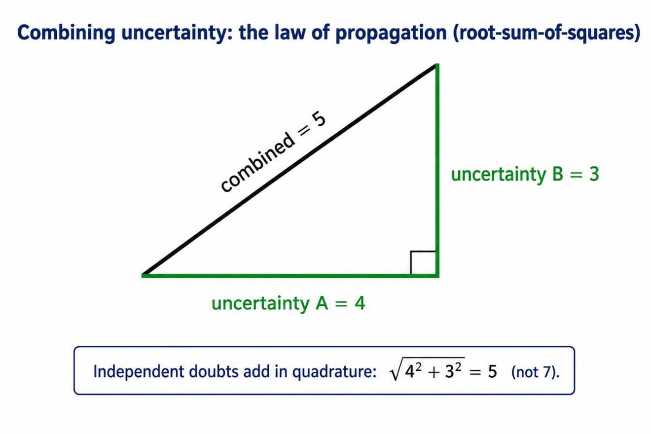
Figure 9. Doubt adds like the sides of a right triangle. Independent uncertainties of 3 and 4 combine to 5, not 7.

Doubt does not add like money. It adds up like the sides of a right triangle. Two uncertainties of 3 and 4 combine not to 7 but to 5, the square root of 3 squared plus 4 squared. This is the root-sum-of-squares, and it is the heart of what the GUM calls the law of propagation of uncertainty (GUM 5.1.2). The reason is that independent doubts partly cancel: when one input happens to read high, another is as likely to read low, so the total grows more slowly than a straight sum.

Before you square and add, though, every piece has to be in the same units, the units of the result. A temperature uncertainty in degrees Celsius cannot be added to a force uncertainty in pounds until you convert it. The converter is the sensitivity coefficient: how much the result moves when one input moves by one unit (GUM 5.1.3).

You already used one. In Part 4 we turned a temperature bound into 0.043 lbf of force by multiplying degrees by the cell’s temperature coefficient. That coefficient is the sensitivity coefficient. It answers the recipe question: if this one ingredient is off, how far off is the finished dish? A pinch of salt has a small coefficient. A cup of flour has a large one. Get the big-coefficient inputs right and the small ones barely matter.

For our instrument every input is already expressed in pounds of force at the 5000 lbf point, so the sensitivity coefficients are all 1, and the combination is a clean root-sum-of-squares: square each contribution, add them, take the square root. The nine contributions combine to a combined standard uncertainty of u_c = 0.666 lbf.

One number, one sigma, the honest spread of the result. Notice what dominates. Repeatability alone, at 0.58 lbf, accounts for about three-quarters of the total variance. Reference standard stability, at 0.29 lbf, takes most of what is left. Everything else, including the reference standard’s own calibration uncertainty at 0.05 lbf, barely registers once it is squared. That is the root-sum-of-squares telling you exactly where to spend your next effort: hold the force point steadier and shorten the calibration interval on the reference. The small terms are not worth a second look.

When your inputs move together: correlation

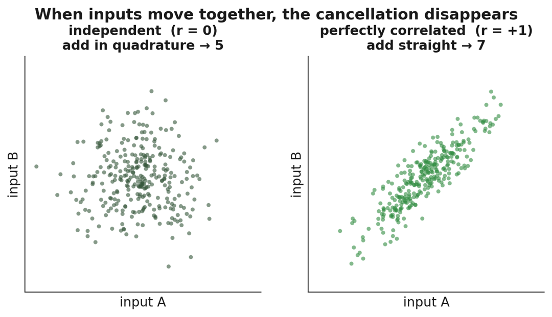
Figure 10. Independent inputs on the left (r = 0) add in quadrature. Perfectly correlated inputs on the right (r = +1) add straight up.

The root-sum-of-squares has a catch, and it is the one most budgets quietly get wrong. It works only when the inputs are independent. When two inputs move together, the partial cancellation that makes doubt add slowly stops happening, and the real uncertainty is larger than the square-root sum.

Two readings are correlated when something they share makes them drift the same way. Measure two forces with the same reference whose value is slightly off, and both readings are off in the same direction by the same fraction. Read two channels through the same thermometer that is reading 0.5 °C high, and both temperature corrections lean the same way. The shared cause links them (GUM 5.2.2).

The GUM measures the link with a correlation coefficient, a number from −1 to +1 (GUM 5.2.2). Zero means independent, and you are back to plain root-sum-of-squares. Plus one means the two move in perfect lockstep. The extreme case is the one to remember, because it sets the worst-case penalty. When two components are perfectly correlated, they no longer add in quadrature. They add straight up, in a simple sum (GUM 5.2.2). That is the difference between 3 and 4 combining to 5 when they are independent and combining to 7 when they are locked together. Correlation can cost you the whole cancellation.

In our single-point budget the nine inputs are effectively independent, so plain root-sum-of-squares holds and u_c stays 0.666 lbf. But the moment you reuse one reference across several force points, or one thermometer across several channels, the correlation is real and you owe it an honest accounting. The practical fix is usually the cleanest one: remove the shared cause, and the correlation goes with it.

Since 2008: the root-sum-of-squares method taught here now carries a formal name. The JCGM calls it the GUM uncertainty framework, or GUF, to set it apart from the Monte Carlo method of Supplement 1 (JCGM 101:2008), which propagates the whole distributions rather than combining standard uncertainties. Both are current. Part 6 shows the day the GUF stops being enough.

Coming in Part 6: we have one honest sigma. Now we stretch it into an interval a customer can act on, and meet the coverage factor. Then the Jaws moment: you head out with k = 2 because it is the boat tied to every dock, look over the side at how little data holds up your biggest term, and realize you are going to need a bigger boat.

-Henry Zumbrun, Morehouse Instrument Company

Appendix: the formulas

Symbols are italic for quantities (U, k, u, s, n) and roman for units (N, kN, lbf). The combined standard uncertainty is u_c, and degrees of freedom is ν.

Standard uncertainty from repeated readings (Type A). For n repeated readings with experimental standard deviation s, the dispersion of a single reading is s itself; the standard uncertainty of their mean is u = s / √n. In force calibration, the repeatability carried is usually s, the doubt in a single determination, not s / √n.

Type B from a stated coverage factor. u = U / k.

Type B from a bound of half-width a. Rectangular: u = a / √3. Triangular: u = a / √6. Normal 99.73 % bound: u = a / 3. Normal 95.45 % bound: u = a / 2. U-shaped: u = a / √2.

Combined standard uncertainty. For independent inputs, root-sum-of-squares: u_c(y) = √[ Σ ( ci × u(xi) )² ]. With correlation, add a covariance term under the root; for perfectly correlated inputs the result reduces to a straight sum.

Expanded uncertainty. U = k × u_c(y).

Effective degrees of freedom (Welch-Satterthwaite). ν_eff = u_c(y)⁴ / Σ [ ui(y)⁴ / νi ]. Truncate to the next lower integer, then take k as the t value at your confidence level for that ν_eff.

Selected t values at 95 % confidence (NIST Technical Note 1297, Table B.1).

Worked combination for the running example. u_c = √(0.58² + 0.29² + 0.10² + 0.087² + 0.05² + 0.043² + 0.032² + 0.0029² + 0.006²) lbf = 0.666 lbf. The fourth-power sum is dominated by repeatability, 0.58⁴ / 3, so ν_eff ≈ 5.2, truncated to 5. U = 2.57 × 0.666 lbf = 1.71 lbf (0.0342 %).

References for the series: JCGM 100:2008 (the GUM) and Amendment 1:2026; JCGM 101:2008 (Monte Carlo); JCGM GUM-5:2026 (examples); JCGM 200:2012 (the VIM); NIST Technical Note 1297 (1994); ISO/IEC 17025:2017, Clauses 7.6 and 7.8.6; ASTM E74; UKAS M3003 Edition 6 (2024); NIST SP 811 (2008).

About Morehouse   

We believe in changing how people think about Force and Torque calibration in everything we do, including, "The GUM in Plain English, Part 5 of 7: Combined Standard Uncertainty: The Catch Called Correlation"

This includes setting expectations and challenging the "just calibrate it" mentality by educating our customers on what matters and what may cause significant errors. 

We focus on reducing these errors and making our products simple and user-friendly. 

This means your instruments will pass calibration more often and produce more precise measurements, giving you the confidence to focus on your business. 

Companies around the globe rely on Morehouse for accuracy and speed. 

Our measurement uncertainties are 10-50 times lower than the competition, providing you with more accuracy and precision in force measurement. 

We turn around your equipment in 7-10 business days so you can return to work quickly and save money. 

When you choose Morehouse, you're not just paying for a calibration service or a load cell. 

You're investing in peace of mind, knowing your equipment is calibrated accurately and on time. 

Through Great People, Great Leaders, and Great Equipment, we empower organizations to make Better Measurements that enhance quality, reduce risk, and drive innovation. 

With over a century of experience, we're committed to raising industry standards, fostering collaboration, helping with understanding risk, and delivering exceptional calibration solutions that build a safer, more accurate future. 

Contact Morehouse at info@mhforce.com to learn more about our calibration services and load cell products. 

Email us if you ever want to chat or have questions about a blog. 

We love talking about this stuff. We have many more topics other than, "The GUM in Plain English, Part 5 of 7: Combined Standard Uncertainty: The Catch Called Correlation"

Our YouTube channel has videos on various force and torque calibration topics here.