The GUM in Plain English, Part 6 of 7: Coverage Factor: Why k = 2 Sometimes Lies

Part 5 combined our nine inputs into a combined standard uncertainty of u_c = 0.666 lbf. That is one sigma, and by itself, it is too thin to act on.

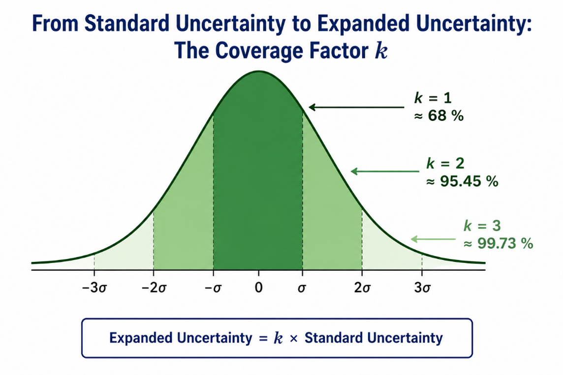
Figure 11. One sigma catches about 68 %. Widen to k = 2 for about 95 %, to k = 3 for about 99 %.

A one-sigma interval catches only about 68 % of where the value could be, which means it misses almost a third of the time. Nobody ships a tolerance on a coin flip plus a bit.

So you widen it. Multiply the combined standard uncertainty by a coverage factor, called k, and you get the expanded uncertainty U (GUM 6.2.1). The interval y ± U is meant to capture a large stated fraction of where the value could reasonably lie. Stretch to k = 2, and you catch about 95 %. Stretch to k = 3, and you catch about 99 % (GUM 6.3.3).

Two things about that multiply are easy to miss, and both matter. First, multiplying by k adds no new information. It only presents the doubt you already had in a more usable form (GUM 6.2.3). The honesty of your U is never better than the u_c underneath it. A confident-looking k = 2 on a sloppy budget is still a sloppy budget. Second, the bare number means nothing without its label. U = 1.71 lbf is not a result. U = 1.71 lbf, k = 2.57, approximately 95 % confidence is the result. Without k and the coverage probability, the next person cannot recover your one-sigma number to combine with theirs. State k every time (GUM 7.2.3).

For our instrument, the comfortable move is U = 2 × 0.666 lbf = 1.33 lbf, k = 2, approximately 95 % confidence. Comfortable, and, as the rest of this part shows, not quite honest. The k = 2 shortcut comes with a condition almost nobody checks.

This is the Jaws moment. You head out with k = 2 because it is the boat tied to every dock. Then you look over the side at how little data is holding your largest term up, and the line writes itself: you are going to need a bigger boat. For our instrument, the bigger boat is k = 2.57. Here is why k = 2 was never big enough.

Effective degrees of freedom, or why k = 2 sometimes lies

Figure 12. The 95 % coverage factor against effective degrees of freedom. Our budget lands at νeff = 5, where k = 2.57, not 2.

Ask a baseball fan whether a hitter batting 0.400 is better than one batting 0.250, and the answer comes fast. Ask whether a player who went 2 for 5 last night is better than one who went 60 for 240 on the season, and the fan slows down. Two hits in five tries tells you almost nothing. Sixty in two hundred forty tells you a lot. Your uncertainty budget has the same problem, and most people never see it.

Every standard uncertainty carries a second number you rarely write down, its degrees of freedom. Think of it as how many independent looks you got before you trusted the spread. Weigh a part twice, and you barely know its scatter. Weigh it fifty times, and you know it well. Degrees of freedom is the bookkeeping for how much you should trust the uncertainty you just calculated.

For a Type A component the rule is simple: if you took n readings, the degrees of freedom is n − 1. Our four repeatability runs give 3. For a Type B component, you assign a large value because you are not going to second-guess a certificate or a resolution limit run to run. The Morehouse budget uses 200 for the Type B pieces, which is large enough that they barely impact the result.

So why does any of this matter? It matters because k = 2 is a promise with a condition. When your combined standard uncertainty is built from components you know well, and the result is roughly normal, then k = 2 buys you about 95 % (GUM 6.3.3). That is the comfortable case. But when a small-sample Type A component dominates the budget, you do not know u_c as well as k = 2 assumes. You calculated a spread from a handful of numbers. The honest interval has to be wider, and the multiplier has to be bigger than 2.

How much bigger? That is the one question the Welch-Satterthwaite formula answers, and it is the part NIST Technical Note 1297 leaves you to look up. In plain language: take each component’s contribution to the combined uncertainty, raise it to the fourth power, divide by that component’s degrees of freedom, and add those up. Divide the fourth power of the total by that sum. The result is the effective degrees of freedom of the whole budget (GUM G.4.1).

The fourth power is the part to feel. It is brutal. It means the largest, least-trusted component sets the answer almost by itself. A big component you measured four times will swamp a dozen small components you know cold.

Watch it land on our running budget. Repeatability is both the largest contribution, at 0.58 lbf, and the least-trusted, resting on only four runs and 3 degrees of freedom. Everything else all but disappears under the fourth power. Run the numbers, and the effective degrees of freedom comes to about 5.2. Truncate to the next lower integer, and you have 5. Now look up the t-value for 95 % confidence at 5 degrees of freedom. It is 2.57, not 2.00.

That gap is the whole point. Report U = 2 × 0.666 lbf = 1.33 lbf, and you have quietly claimed more confidence than your data supports. The honest number is U = 1.71 lbf, k = 2.57, approximately 95 % confidence, nearly 30 % more interval than the lazy version. You only see that cost if you carry the degrees of freedom, and you only shrink it by taking more than four runs at the points that matter.

This is where the ASTM E74 question from Part 3 comes home. Run a full E74 calibration and repeatability does not rest on four runs at one point. It rests on the fit across the whole range, roughly 33 points and 32 degrees of freedom. Rely on the E74 fit for your repeatability, and the dominant term would carry 32 degrees of freedom rather than 3; ν_eff would climb and k would settle back near 2. We did not do that here. We sized repeatability from a single-point sample on purpose, because that is the doubt in one determination at 5000 lbf, and the price of that honesty is ν_eff = 5 and k = 2.57. Same instrument, same machine, two defensible numbers. The only difference is how much data you let stand behind the term that dominates, and you should always know which one you are reporting.

Simple, right? So carry them. Put a degrees-of-freedom column in every budget you build. When the effective degrees of freedom comes back large, use k = 2 and move on. When it comes back small, reach for the t table and tell the truth.

There is a second way k = 2 can lie, and it runs in the opposite direction. Welch-Satterthwaite handles a small-sample Type A term that dominates. But sometimes the term that dominates is Type B and rectangular, most often a coarse indicator resolution whose half-step bound swamps everything else. When that happens, the combined result is no longer normal, and k = 2 over-claims instead of under-claiming (M3003 Appendix C). M3003 gives a quick test: divide the standard uncertainty of all the remaining terms by the standard uncertainty of the dominant rectangular term. If that ratio falls below 0.70, the rectangular term sets the shape, and you read the coverage factor from a convolution table rather than the t table. For a budget that is almost purely rectangular, the 95 % factor falls to about 1.65, not 2. Our running budget is safe here, because the largest term is repeatability, a Type A piece that behaves normally. On an instrument with coarse resolution, run the test before you trust k = 2.

Since 2008: the escape hatch at the end of this part is now a full method. When the effective degrees of freedom machinery, the GUF, breaks down, JCGM 101:2008 propagates the input distributions by Monte Carlo and reads the coverage interval straight off the result, with no Welch-Satterthwaite and no t table. You will rarely need it for a force budget. It is the JCGM’s own answer when k cannot be trusted at all. And as of 2026 the advice sits in the GUM itself: Amendment 1 (JCGM 100:2008/Amd.1:2026) adds a note at 4.1.4 that when nonlinearity is significant, you either carry the higher-order Taylor terms or go straight to the Monte Carlo of JCGM 101.

Coming in Part 7: the finish line. How to report a result so a competent stranger can rebuild it, the conformity-statement trap that gets labs written up, and the complete 5000 lbf budget on one page, from four noisy readings all the way to U = 1.71 lbf, k = 2.57.

-Henry Zumbrun, Morehouse Instrument Company

Appendix: the formulas

Symbols are italic for quantities (U, k, u, s, n) and roman for units (N, kN, lbf). The combined standard uncertainty is u_c, and degrees of freedom is ν.

Standard uncertainty from repeated readings (Type A). For n repeated readings with experimental standard deviation s, the dispersion of a single reading is s itself; the standard uncertainty of their mean is u = s / √n. In force calibration, the repeatability carried is usually s, the doubt in a single determination, not s / √n.

Type B from a stated coverage factor. u = U / k.

Type B from a bound of half-width a. Rectangular: u = a / √3. Triangular: u = a / √6. Normal 99.73 % bound: u = a / 3. Normal 95.45 % bound: u = a / 2. U-shaped: u = a / √2.

Combined standard uncertainty. For independent inputs, root-sum-of-squares: u_c(y) = √[ Σ ( ci × u(xi) )² ]. With correlation, add a covariance term under the root; for perfectly correlated inputs the result reduces to a straight sum.

Expanded uncertainty. U = k × u_c(y).

Effective degrees of freedom (Welch-Satterthwaite). ν_eff = u_c(y)⁴ / Σ [ ui(y)⁴ / νi ]. Truncate to the next lower integer, then take k as the t value at your confidence level for that ν_eff.

Selected t values at 95 % confidence (NIST Technical Note 1297, Table B.1).

Worked combination for the running example. u_c = √(0.58² + 0.29² + 0.10² + 0.087² + 0.05² + 0.043² + 0.032² + 0.0029² + 0.006²) lbf = 0.666 lbf. The fourth-power sum is dominated by repeatability, 0.58⁴ / 3, so ν_eff ≈ 5.2, truncated to 5. U = 2.57 × 0.666 lbf = 1.71 lbf (0.0342 %).

References for the series: JCGM 100:2008 (the GUM) and Amendment 1:2026; JCGM 101:2008 (Monte Carlo); JCGM GUM-5:2026 (examples); JCGM 200:2012 (the VIM); NIST Technical Note 1297 (1994); ISO/IEC 17025:2017, Clauses 7.6 and 7.8.6; ASTM E74; UKAS M3003 Edition 6 (2024); NIST SP 811 (2008).

About Morehouse   

We believe in changing how people think about Force and Torque calibration in everything we do, including, "The GUM in Plain English, Part 6 of 7: Coverage Factor: Why k = 2 Sometimes Lies"

This includes setting expectations and challenging the "just calibrate it" mentality by educating our customers on what matters and what may cause significant errors. 

We focus on reducing these errors and making our products simple and user-friendly. 

This means your instruments will pass calibration more often and produce more precise measurements, giving you the confidence to focus on your business. 

Companies around the globe rely on Morehouse for accuracy and speed. 

Our measurement uncertainties are 10-50 times lower than the competition, providing you with more accuracy and precision in force measurement. 

We turn around your equipment in 7-10 business days so you can return to work quickly and save money. 

When you choose Morehouse, you're not just paying for a calibration service or a load cell. 

You're investing in peace of mind, knowing your equipment is calibrated accurately and on time. 

Through Great People, Great Leaders, and Great Equipment, we empower organizations to make Better Measurements that enhance quality, reduce risk, and drive innovation. 

With over a century of experience, we're committed to raising industry standards, fostering collaboration, helping with understanding risk, and delivering exceptional calibration solutions that build a safer, more accurate future. 

Contact Morehouse at info@mhforce.com to learn more about our calibration services and load cell products. 

Email us if you ever want to chat or have questions about a blog. 

We love talking about this stuff. We have many more topics other than, "The GUM in Plain English, Part 6 of 7: Coverage Factor: Why k = 2 Sometimes Lies"

Our YouTube channel has videos on various force and torque calibration topics here.